In this scenario, we have a continuous \(M\), a binary outcome \(Y\), and an effect modifier on \(Y\), x2. The sample size is 50
and there are 3 covariates.
Sample simulated Dataset
Example with N=50, L=3 for scenario 4 (binary \(Y\), continuous \(M\), x2 is an effect modifier
on \(Y\)):
dat <-  cma_sampledata(N = 50, L=3, P=3, scenario=1, seed=7)
head(dat$data, n = 3L)
#>           z1         z2         z3           M         x1          x2        x3
#> 1  2.2767428  0.1432685  0.7973699  0.58827130 -0.3556944  2.02334405 -1.477592
#> 2 -1.0893537 -0.0944783  0.4035083  0.01382552  1.0973004  0.86249250 -2.973256
#> 3 -0.6389109  0.2491581 -0.1243989 -0.42344188 -0.9066920 -0.02490949 -1.339762
#>           y
#> 1  1.964451
#> 2 -1.526532
#> 3 -1.305984
dat = dat$data
Fit BKMR Models
let \(A\) be a \(n\)-by-\(L\) matrix containing an exposure mixture
comprised of \(L\)
elements,E.M and E.Y be effect modifiers of
exposure-mediator and exposure-outcome relationship respectively, \(y\), a vector of outcome data, and \(m\), a vector of mediator data.
Z.M <- cbind(A,E.M)
Z.Y <- cbind(A,E.Y)
Let Z.M be the exposures and effect modifers
E.M and let Z.Y be the exposures and effect
modifers E.Y, create one more matrix containing the
exposures, effect modifier Z.Y and mediator, precisely in
that order.
Zm.Y <- cbind(Z.Y,m)
NOTE: the last column of the Zm.Y matrix must
be your mediator in order for the functions to work properly.
A <- cbind(dat$z1, dat$z2, dat$z3)
X <- cbind(dat$x1, dat$x2, dat$x3)
y  <- dat$y
m  <- dat$M

E.M <- NULL
E.Y <- dat$x2

Z.M <- cbind(A,E.M)
Z.Y <- cbind(A, E.Y)
Zm.Y <- cbind(Z.Y, m)

set.seed(1)
fit.y <- kmbayes(y=y, Z=Zm.Y, X=X, iter=10000, verbose=TRUE, varsel=FALSE)
#save(fit.y,file="bkmr_y.RData")

set.seed(2)
fit.y.TE <- kmbayes(y=y, Z=Z.Y, X=X, iter=10000, verbose=TRUE, varsel=FALSE)
#save(fit.y.TE,file="bkmr_y_TE.RData")

set.seed(3)
fit.m <- kmbayes(y=m, Z=Z.M, X=X, iter=10000, verbose=TRUE, varsel=FALSE)
#save(fit.m,file="bkmr_m.RData")
Values at which to predict counterfactuals
Mean level of confounders:
We define the change in exposure for which you want to estimate the
mediation effects: in this example, we will consider a change in all
exposures from their 25th to 75th percentiles, fixing age
(E.Y) at testing to its 10th and 90th percentiles. However,
this contrast can be anything.
Note: If modifiers are considered, you should fix the levels of the modifiers
astar <- c(apply(A, 2, quantile, probs=0.25))
a <- c(apply(A, 2, quantile, probs=0.75))

e.y10 = quantile(E.Y, probs=0.1)
e.y90 = quantile(E.Y, probs=0.9)
The index of the MCMC iterations to be used for inference:
sel<-seq(5000,10000,by=10)Estimate TE for BKMR
Estimate the TE for a change in the exposures from \(a^*\) to \(a\) fixing Effect modifier at testing to its 10th percentile or 90th percentile:
e.y10 = quantile(E.Y, probs=0.1)
e.y90 = quantile(E.Y, probs=0.9)

TE.ey10 <- TE.bkmr(a=a, astar=astar, e.y = e.y10, fit.y.TE=fit.y.TE, X.predict=X.predict, alpha=0.05, sel=sel, seed=122)

TE.ey90 <- TE.bkmr(a=a, astar=astar, e.y = e.y90, fit.y.TE=fit.y.TE, X.predict=X.predict, alpha=0.05, sel=sel, seed=122)
Look at the posterior mean, median, and 95% CI for TE:
TE.ey10$est
#>         mean    median     lower    upper        sd
#> TE 0.4433419 0.4451366 0.2863908 0.601123 0.0802884
TE.ey90$est
#>        mean   median    lower    upper         sd
#> TE 1.339359 1.343762 1.179134 1.477626 0.07874423

plotdf <- as.data.frame(TE.ey10$est)
plotdf["Effect"] <- rownames(plotdf)
ggplot(plotdf, aes(Effect, mean, ymin = lower, ymax = upper))  +
  geom_pointrange(position = position_dodge(width = 0.75))  +  coord_flip()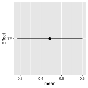
Estimate CDE for BKMR
Estimate the CDE for a change in the exposures from \(a^*\) to \(a\), fixing the mediator at its 10th, 50th, and 75th percentile and the effect modifier at testing at its 10th percentile:
CDE.ey10 <- CDE.bkmr(a=a, astar=astar, e.y = e.y10, m.quant=c(0.1,0.5,0.75), fit.y=fit.y, alpha=0.05, sel=sel, seed=777)
#> [1] "Running 3 mediator values for CDE:"
#> [1] "1 out of 3"
#> [1] "2 out of 3"
#> [1] "3 out of 3"

CDE.ey90 <- CDE.bkmr(a=a, astar=astar, e.y = e.y90, m.quant=c(0.1,0.5,0.75), fit.y=fit.y, alpha=0.05, sel=sel, seed=777)
#> [1] "Running 3 mediator values for CDE:"
#> [1] "1 out of 3"
#> [1] "2 out of 3"
#> [1] "3 out of 3"
Look at the posterior mean, median, and 95% CI for the CDEs:
CDE.ey10$est
#>             mean    median     lower     upper         sd
#> CDE10% 0.3260377 0.3276014 0.1254467 0.5072569 0.10005344
#> CDE50% 0.3478852 0.3488510 0.1461287 0.5280398 0.09656925
#> CDE75% 0.3581060 0.3617068 0.1598766 0.5443135 0.10011163
CDE.ey90$est
#>            mean   median     lower    upper         sd
#> CDE10% 1.215059 1.220603 0.9850737 1.413276 0.10774925
#> CDE50% 1.233969 1.237500 1.0434691 1.410319 0.09388749
#> CDE75% 1.238180 1.244269 1.0387424 1.408041 0.09410765
Plotting:
plotdf <- as.data.frame(CDE.ey10$est)
plotdf["Effect"] <- rownames(plotdf)
ggplot(plotdf, aes(Effect, mean, ymin = lower, ymax = upper ))  +
  geom_pointrange(position = position_dodge(width = 0.75))  +  coord_flip()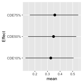
Estimate NDE/NIE for BKMR
Estimate the TE, NDE and NIE for a change in the exposures from \(a^*\) to \(a\) fixing age at testing to its 90th percentile.
Note: this step takes a while to run and will take longer for more
complex BKMR fits, longer sel vectors and larger.
mediationeffects.ey10  <- mediation.bkmr(a=a, astar=astar, e.y = e.y10, fit.m=fit.m, fit.y=fit.y, fit.y.TE=fit.y.TE, X.predict.M=X.predict, X.predict.Y=X.predict, alpha=0.05, sel=sel, seed=22, K=10)

mediationeffects.ey90  <- mediation.bkmr(a=a, astar=astar, e.y = e.y90, fit.m=fit.m, fit.y=fit.y, fit.y.TE=fit.y.TE, X.predict.M=X.predict, X.predict.Y=X.predict, alpha=0.05, sel=sel, seed=22, K=10)
Look at the posterior mean, median, and 95% CI for the TE, NDE, and NIE
mediationeffects.ey10$est
#>               mean      median       lower     upper         sd
#> TE      0.43475329  0.43695477  0.28272467 0.5967626 0.07940782
#> NDE     0.46065802  0.45305129 -0.02506667 0.9820913 0.25342409
#> NIE    -0.02590473 -0.02825869 -0.54095110 0.4387311 0.25652203
#> CDE10%  0.31667148  0.31721110  0.09980919 0.4998968 0.09934223
#> CDE50%  0.33851356  0.33967494  0.13406825 0.5088642 0.09641575
#> CDE75%  0.34827973  0.35279634  0.12335966 0.5288362 0.10060523
mediationeffects.ey90$est
#>              mean     median      lower     upper         sd
#> TE     1.33176656 1.33620159  1.1664505 1.4777750 0.07597909
#> NDE    1.30990305 1.30828526  0.7755002 1.8451772 0.27812748
#> NIE    0.02186351 0.01546491 -0.5021909 0.5836256 0.27216157
#> CDE10% 1.20566661 1.20823512  0.9692586 1.4128013 0.10788303
#> CDE50% 1.22551431 1.22766297  1.0196915 1.3944634 0.09285689
#> CDE75% 1.22965520 1.23325711  1.0226156 1.3937021 0.09261384
Plotting
plotdf <- as.data.frame(mediationeffects.ey10$est)
plotdf["Effect"] <- rownames(plotdf)
ggplot(plotdf, aes(Effect, mean, ymin = lower, ymax = upper ))  +
  geom_pointrange(position = position_dodge(width = 0.75))  +  coord_flip()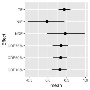
Summary statistics of the predictor-response function
Risk Summary For Totel Effect
riskSummary10 = TERiskSummaries.CMA(fit.TE = fit.y.TE, e.y=e.y10, e.y.name = "E.Y", sel=sel)

ggplot(riskSummary10,
       aes(quantile,
           est,
           ymin = est - 1.96 * sd,
           ymax = est + 1.96 * sd)) +
  geom_pointrange()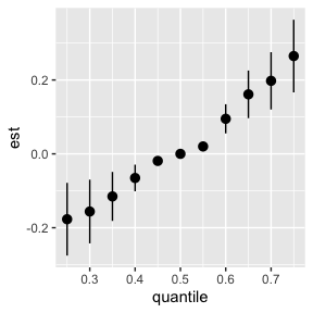
riskSummary90 = TERiskSummaries.CMA(fit.TE = fit.y.TE, e.y=e.y90, e.y.name = "E.Y", sel=sel)

ggplot(riskSummary90,
       aes(quantile,
           est,
           ymin = est - 1.96 * sd,
           ymax = est + 1.96 * sd)) +
  geom_pointrange()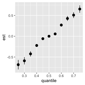
Risk Summary For Controlled Direct Effect
# CDE
CDEriskSummary10 = CDERiskSummaries.CMA(fit.y = fit.y, e.y = e.y10, e.y.name = "E.Y", m.name = "m", sel = sel)
ggplot(CDEriskSummary10, aes(quantile, est, ymin = est - 1.96*sd,
                             ymax = est + 1.96*sd, col = m)) +
  geom_pointrange(position = position_dodge(width = 0.75))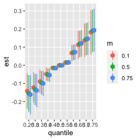
CDEriskSummary90 = CDERiskSummaries.CMA(fit.y = fit.y, e.y = e.y90, e.y.name = "E.Y", m.name = "m", sel = sel)
ggplot(CDEriskSummary90, aes(quantile, est, ymin = est - 1.96*sd,
                             ymax = est + 1.96*sd, col = m)) +
  geom_pointrange(position = position_dodge(width = 0.75))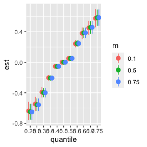
Single-predictor health risks
Total Effect
risks.singvar10 = SingVarRiskSummaries.CMA(BKMRfits = fit.y.TE, which.z = 1:3,
                                           e.y=e.y10, e.y.names="E.Y",
                                           sel=sel)
ggplot(risks.singvar10, aes(variable, est, ymin = est - 1.96*sd,
                            ymax = est + 1.96*sd, col = q.fixed)) +
  geom_pointrange(position = position_dodge(width = 0.75)) +
  coord_flip()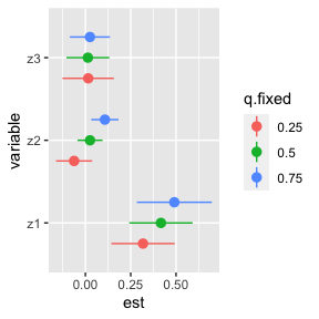
risks.singvar90 = SingVarRiskSummaries.CMA(BKMRfits = fit.y.TE, which.z = 1:3,
                                           e.y=e.y90, e.y.names="E.Y",
                                           sel=sel)
ggplot(risks.singvar90, aes(variable, est, ymin = est - 1.96*sd,
                            ymax = est + 1.96*sd, col = q.fixed)) +
  geom_pointrange(position = position_dodge(width = 0.75)) +
  coord_flip()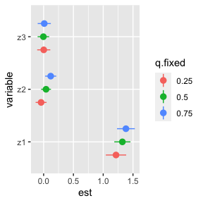
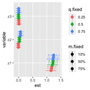
Controlled Direct Effect
# single variable controlled direct effects
CDErisks.singvar10 = CDESingVarRiskSummaries.CMA(BKMRfits = fit.y,
                                           e.y=e.y10, e.y.names="E.Y", m.name = "m",
                                           sel=sel)
ggplot(CDErisks.singvar10, aes(variable, est, ymin = est - 1.96*sd,
                            ymax = est + 1.96*sd, col = q.fixed, linetype = m.fixed)) +
  geom_pointrange(position = position_dodge(width = 0.75)) +
  coord_flip()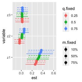
CDErisks.singvar90 = CDESingVarRiskSummaries.CMA(BKMRfits = fit.y,
                                                 e.y=e.y90, e.y.names="E.Y", m.name = "m",
                                                 sel=sel)
ggplot(CDErisks.singvar90, aes(variable, est, ymin = est - 1.96*sd,
                               ymax = est + 1.96*sd, col = q.fixed, linetype = m.fixed)) +
  geom_pointrange(position = position_dodge(width = 0.75)) +
  coord_flip()