Causal Estimands
We consider a setting in which \(n\) subjects, labelled \(i = 1, ..., n\), enter a study at baseline (time \(t=0\)) and are subjected to treatment \(A_{0, i}\). In a clinical trial, the value of \(A_{0, i}\) is determined by the study protocol, usually at random. In an observational study, \(A_{0, i}\) is observed and recorded. A collection of covariates, \(C_{0, i}\), are also measured at baseline. At the subsequent follow-up visits, the time-varying confounders, \(L_{t, i}\) and treatment \(A_{t, i}\) are recorded, \(t = 1, ..., T\). An outcome \(Y_i\) is observed for each subject, measured at the final visit \(T\), \(Y_i\) can be continuous or binary.
Along with the \(Y_i\) for each subject, for each possible realization of the treatment history \(\bar{a} \in \bar{\mathcal{A}}\); we also define \(Y_i^{\bar{a}}\), the that would have been observed had the subject, possibly contrary to fact, received treatment history \(\bar{a}\).
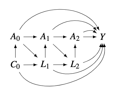
In a simple setting with 3 visits, assume the following DAG. Under the static, fixed treatment regimes, the overall causal effect of the exposures changing form the \(25^{th}\) percentile to the \(75^{th}\) percentile can be defined as:
\[ACE = E[Y^{A_0 = a_0^*, A_1 = a_1^*, A_2 = a_2^*}] - E[Y^{A_0 = a_0, A_1 = a_1, A_2 = a_2}]\] where \(a_0, a_1, a_2\) are the \(25^{th}\) percentile of the exposures, \(a_0^*, a_1^*, a_2^*\) are the \(75^{th}\) percentile of the exposures.
g-formula
The basic idea of g-formula is standardization, a common approach to estimating the expected value of \(Y^{\bar{a}}\) in the population. (Naimai, Ashley I., et al., 2017) It can be illustrated in a simple time-fixed confounding example where there are only baseline confounders \(C_0\) where the sum is over all possible values \(c_0\) of \(C_0\). \[E\left(Y^{\bar{a}}\right)=\sum_{C_{0} } E\left(Y \mid \bar{A}=\bar{a}, C_{0}=c_{0}\right) P\left(C_{0}=c_{0}\right)\] where the sum is over all possible values \(c_0\) of \(C_0\).\
Using the above DAG, we now define 3 identifying assumptions:\
Consistency: \[E[Y | A_0 = a_0, A_1 = a_1, A_2 = a_2] = E[Y^{a_0, a_1, a_2}| A_0 = a_0, A_1 = a_1, A_2 = a_2]\]
Exchangeability:
Positivity: \[Pr(a_t|a_{t-1}, l_t, c_0) > 0 \ \text{for all values of} \ l \ \text{with} \ Pr(L = l) \ne 0 \]
The general expression of the g-formula for a static fixed intervention is: \[\begin{equation} E[Y^{\bar{a}}]= \sum_{\bar{l}} \mathrm{E}[Y \mid \bar{A}=\bar{a}, \bar{L}=\bar{l}, C_0 = c_0] \prod_{t=0}^{T} f\left(l_{t} \mid \bar{a}_{t-1}, \bar{l}_{t-1} \right)f(c_0) \end{equation}] \]
Bayesian kernel machine regression
We first review Kernel Machine Regression (KMR) as a framework for estimating the effect of a complex mixture when only a single time point of exposure is measured. For each subject \(i = 1, ..., n\), we assume
\[\begin{equation} Y_{i}=h\left(\mathbf{a}_{i}\right)+\mathbf{c}_{i}^{\mathrm{T}} \boldsymbol{\beta}+\epsilon_{i} \end{equation}\] where \(\mathbf{a}_{i}=\left(a_{i 1}, \ldots, a_{i M}\right)^{\mathrm{T}}\) is a vector of \(M\) exposure variables.
It can be shown that the above model can be expressed as the mixed model \[y_{i} \sim N\left(h_{i}+\mathbf{c}_{i}^{T} \boldsymbol{\beta}, \sigma^{2}\right)\]
\[\begin{equation} \mathbf{h} \equiv\left(h_{1}, \ldots, h_{n}\right)^{\mathrm{T}} \sim N(\mathbf{0}, \tau \mathbf{K}) \end{equation}\]
where \(\mathbf{K}\) is the kernel matrix, has \((i, j)-\)element \(K(\mathbf{a}_{i}, \mathbf{a}_{j})\)
There are different choices of the kernel. We focus on the Gaussian kernel, which flexibly captures a wide range of underlying functional forms for \(h(\cdot)\), although the methods are applicable to a broad choice of kernels. We assume \[\operatorname{cor}\left(h_{i}, h_{j}\right)=\exp \left\{-(1 / \rho) \sum_{m=1}^{M}\left(a_{i m}-a_{j m}\right)^{2}\right\}\] where \(\rho\) is a tuning parameter that regulates the smoothness of the dose-response function. This assumption implies that two subjects with similar exposures will have more similar risks (\(a_i\) to \(a_j\), and \(h_i\) will be close to \(h_j\) ).
Bobb et al (2015) presented the Bayesian Kernel Machine Regression (BKMR) as a framework to estimate the effect of a complex mixture on a health outcome.
To fit (2), we assume a at prior on the coefficients for the
confounding variables, \(\beta \sim
1\), and
\(\sigma^{-2} \sim
\operatorname{Gamma}\left(a_{\sigma}, b_{\sigma}\right)\), where
we set \(a_{\sigma} = b_{\sigma} =
0.001\).
We can parameterize BKMR by \(\lambda=\tau \sigma^{-2}\), and we assume a Gamma prior distribution for the variance component of \(\lambda\). For the smoothness parameter \(\rho\), we assume \(\rho \sim \operatorname{Unif}(a, b)\) with \(a=0\) and \(b=100\). For additional details regarding BKMR and prior specifications, see Bobb et al. (Bobb et al., 2015, 2018)
References
Anglen Bauer J, Devick KL, Bobb JF, Coull BA, Zoni S, Fedrighi C, Benedetti C, Guazzetti S, White R, Bellinger D, Yang Q, Webster T, Wright RO, Smith D, Lucchini R, Claus Henn. Associations from a mixture of manganese, lead, copper and chromium and adolescent neurobehavior.
Bobb JF, Claus Henn B, Valeri L, Coull BA. 2018. Statistical software for analyzing the health effects of multiple concurrent exposures via Bayesian kernel machine regression. Environ Health 17:67; doi:10.1186/s12940-018-0413-y.
Bobb JF, Valeri L, Claus Henn B, Christiani DC, Wright RO, Mazumdar M, et al. 2015. Bayesian kernel machine regression for estimating the health effects of multi-pollutant mixtures. Biostatistics 16:493–508; doi:10.1093/biostatistics/kxu058.
Rubin DB. 1987. Multiple imputation for nonresponse in surveys. Wiley.
Valeri L, Mazumdar M, Bobb J, Claus Henn B, Sharif O, Al. E. 2017. The joint effect of prenatal exposure to metal mixtures on neurodevelopmental outcomes at 24 months: evidence from rural Bangladesh. Env Heal Perspect 125; doi:DOI: 10.1289/EHP614.